Gender Identification
About The Project
Gender Identification is the task of classifying an audio into gender labels (we used 'male' and 'female'). We needed to identify whether the voice present in each utterance was male or female since it is a very important step while trying to balance your data among gender classes, for any downstream task. This also helps in maintaining diversity in data.
Our intelligent data pipelines split each audio, based on Voice Activity Detection, as one of the starting steps. These shorter audio utterances can then used to train deep learning models. We assume that the utterances are short enough to have one speaker per utterance, since the splitting logic is using unvoiced segments as points to split an audio.
We use embeddings (explained in the next section) to train a machine learning based classifier and achieve an accurracy of 96% on our test set. (Datasets and training explained later.)
Working
Embeddings
To convert our audio utternaces into fixed length summary vectors, we use the Voice Encoder model proposed here, and implemented here for converting our audio utterances into fixed length embeddings.
Voice Encoder is a speaker-discriminative model trained on a text-independent speaker verification task. Since these embeddings are able to summarise the characteristics of the voice spoken, they have been used for Gender Classification here, as shown in the diagram below.
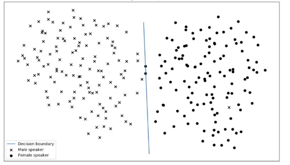
The above plot shows a clear boundary for gender between embeddings from distinct speakers present in LibriSpeech dataset, when projected in 2D using umap.
Classification algorithm
We use the Support vector machine classifier defined here to train for gender classification task, with embeddings from previous step and input, and their correct gender labels as target classes.
Support vector machines (SVMs) are a set of supervised learning methods used for classification, regression and outliers detection.
The advantages of support vector machines are:
-
Effective in high dimensional spaces. Our space is 256 dimensional.
-
Still effective in cases where number of dimensions is greater than the number of samples.
-
Uses a subset of training points in the decision function (called support vectors), so it is also memory efficient.
Hyperparameters
Below is the description of each hyperparameter we used, with the value we used it it.
- kernel: 'rbf'
- RBF Kernel is popular because of its similarity to K-Nearest Neighborhood Algorithm. It has the advantages of K-NN and overcomes the space complexity problem as RBF Kernel Support Vector Machines just needs to store the support vectors during training and not the entire dataset.
When training an SVM with the Radial Basis Function (RBF) kernel, two parameters must be considered: C and gamma. The parameter C, common to all SVM kernels, trades off misclassification of training examples against simplicity of the decision surface. A low C makes the decision surface smooth, while a high C aims at classifying all training examples correctly. gamma defines how much influence a single training example has. The larger gamma is, the closer other examples must be to be affected.
We used the following values for C and gamma: - gamma: 0.01 - C: 100
Train data
We used data for training as a combined set of audios in the following languages: Hindi, Tamil, Telugu, Kannada.
Final train dataset had the following distribution: - male: 17.4 hours - female: 16.2 hours
Test data
We used data for training as a combined set of audios in the following languages: Hindi, Tamil, Telugu, Kannada, Marathi and Bengali. Test data had two additional languages, as compared to the train data: Marathi and Bengali.
Final test dataset (balanced) had the following distribution: - male: 3.6 hours - female: 3.6 hours
Usage
Parameters to change
-
model-path : set the path where you want to save the trained model.
eg: 'path/to/trained/model/model.sav' -
file-mode : default=False; set True for single file inference
- file-path : path to .wav file if --file-mode = True
- csv-path : path to csv containing multiple audio file paths
- save-dir : default= current directory; else give path to save predictions.csv
Commands for Inference
For single file inference:
python scripts/inference.py --model-path model/clf_svc.sav --file-mode True --file-path <filename>.wav
For CSV mode inference:
Create a csv containing multiple file paths
python scripts/inference.py --model-path model/clf_svc.sav --csv-path <file_paths>.csv --save-dir <destination path>